Replicating ProPublica's COMPAS data analysis with Python
Replicating ProPublica’s COMPAS data analysis with Python
In May 2016, a ProPublica article (Angwin et al. 2016) showed the COMPAS Recidivism Algorithm, used by US courts to predict recidivism, is biased against African Americans. The authors offered the codes in R. Based on their codes, I re-produced in Python the first half of ProPublica’s evaluation of the COMPAS Recidivism Algorithm.
1) COMPAS score and risk of recidivism
Load data
import pandas as pd
import numpy as np
pd.options.mode.chained_assignment = None  # default='warn'

dataURL = 'https://raw.githubusercontent.com/propublica/compas-analysis/master/compas-scores-two-years.csv'
dfRaw = pd.read_csv(dataURL)
Select fields for severity of charge, number of priors, demographics, age, sex, compas scores, and whether each person was accused of a crime within two years.
dfFiltered = (dfRaw[['age', 'c_charge_degree', 'race', 'age_cat', 'score_text',
             'sex', 'priors_count', 'days_b_screening_arrest', 'decile_score',
             'is_recid', 'two_year_recid', 'c_jail_in', 'c_jail_out']]
             .loc[(dfRaw['days_b_screening_arrest'] <= 30) & (dfRaw['days_b_screening_arrest'] >= -30), :]
             .loc[dfRaw['is_recid'] != -1, :]
             .loc[dfRaw['c_charge_degree'] != 'O', :]
             .loc[dfRaw['score_text'] != 'N/A', :]
             )
print('Number of rows: {}'.format(len(dfFiltered.index)))
Number of rows: 6172
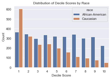
Score distribution by race
The distribution of decile scores, which are often presented to judges alongside risk classification (High, Medium and Low), suggests disparity. There is no clear downtrend in decile scores for African American defendents, unlike for the Caucasian counterpart.
COMPAS scores for each defendant ranged from 1 to 10, with ten being the highest risk. Scores 1 to 4 were labeled by COMPAS as “Low”; 5 to 7 were labeled “Medium”; and 8 to 10 were labeled “High.”
Simple cross tabulation of score categories by race
pd.crosstab(dfFiltered['score_text'],dfFiltered['race'])
| race | African-American | Asian | Caucasian | Hispanic | Native American | Other |
|---|---|---|---|---|---|---|
| High | 845 | 3 | 223 | 47 | 4 | 22 |
| Low | 1346 | 24 | 1407 | 368 | 3 | 273 |
| Medium | 984 | 4 | 473 | 94 | 4 | 48 |
Decile scores that correspond to score categories
pd.crosstab(dfFiltered['score_text'],dfFiltered['decile_score'])
| decile_score | 1 | 2 | 3 | 4 | 5 | 6 | 7 | 8 | 9 | 10 |
|---|---|---|---|---|---|---|---|---|---|---|
| Low | 1286 | 822 | 647 | 666 | 0 | 0 | 0 | 0 | 0 | 0 |
| Medium | 0 | 0 | 0 | 0 | 582 | 529 | 496 | 0 | 0 | 0 |
| High | 0 | 0 | 0 | 0 | 0 | 0 | 0 | 420 | 420 | 304 |
Histograms of decile scores
%matplotlib inline
import seaborn as sns
import matplotlib.pyplot as plt

sns.set(style='darkgrid')
sns.countplot(x='decile_score', hue='race', data=dfFiltered.loc[
                (dfFiltered['race'] == 'African-American') | (dfFiltered['race'] == 'Caucasian'),:
            ])

plt.title("Distribution of Decile Scores by Race")
plt.xlabel('Decile Score')
plt.ylabel('Count')
Text(0, 0.5, 'Count')
Regression analysis - logistic regression
Here, I transform cateogorical data into dummy variables and run logistic regressions that consider race, age, criminal history, future recidivism, charge degree, gender and age. ‘High’ and ‘Medium’ categories are combined following the ProPublica analysis.
import statsmodels.api as sm
from statsmodels.formula.api import logit
catCols = ['score_text','age_cat','sex','race','c_charge_degree']
dfFiltered.loc[:,catCols] = dfFiltered.loc[:,catCols].astype('category')

# dfDummies = pd.get_dummies(data = dfFiltered.loc[dfFiltered['score_text'] != 'Low',:], columns=catCols)
dfDummies = pd.get_dummies(data = dfFiltered, columns=catCols)

# Clean column names
new_column_names = [col.lstrip().rstrip().lower().replace(" ", "_").replace("-", "_") for col in dfDummies.columns]
dfDummies.columns = new_column_names

# We want another variable that combines Medium and High
dfDummies['score_text_medhi'] = dfDummies['score_text_medium'] + dfDummies['score_text_high']
Logistic regression
# R-style specification
formula = 'score_text_medhi ~ sex_female + age_cat_greater_than_45 + age_cat_less_than_25 + race_african_american + race_asian + race_hispanic + race_native_american + race_other + priors_count + c_charge_degree_m + two_year_recid'

score_mod = logit(formula, data = dfDummies).fit()
print(score_mod.summary())
Optimization terminated successfully.
         Current function value: 0.499708
         Iterations 6
                           Logit Regression Results
==============================================================================
Dep. Variable:       score_text_medhi   No. Observations:                 6172
Model:                          Logit   Df Residuals:                     6160
Method:                           MLE   Df Model:                           11
Date:                Sat, 21 Nov 2020   Pseudo R-squ.:                  0.2729
Time:                        16:26:02   Log-Likelihood:                -3084.2
converged:                       True   LL-Null:                       -4241.7
Covariance Type:            nonrobust   LLR p-value:                     0.000
===========================================================================================
                              coef    std err          z      P>|z|      [0.025      0.975]
-------------------------------------------------------------------------------------------
Intercept                  -1.5255      0.079    -19.430      0.000      -1.679      -1.372
sex_female                  0.2213      0.080      2.783      0.005       0.065       0.377
age_cat_greater_than_45    -1.3556      0.099    -13.682      0.000      -1.550      -1.161
age_cat_less_than_25        1.3084      0.076     17.232      0.000       1.160       1.457
race_african_american       0.4772      0.069      6.881      0.000       0.341       0.613
race_asian                 -0.2544      0.478     -0.532      0.595      -1.192       0.683
race_hispanic              -0.4284      0.128     -3.344      0.001      -0.680      -0.177
race_native_american        1.3942      0.766      1.820      0.069      -0.107       2.896
race_other                 -0.8263      0.162     -5.098      0.000      -1.144      -0.509
priors_count                0.2689      0.011     24.221      0.000       0.247       0.291
c_charge_degree_m          -0.3112      0.067     -4.677      0.000      -0.442      -0.181
two_year_recid              0.6859      0.064     10.713      0.000       0.560       0.811
===========================================================================================
Black defendants were 45.3 percent more likely than white defendants to receive a higher score, correcting for prior crimes, future criminality.
control = np.exp(-1.5255) / (1 + np.exp(-1.5255))
np.exp(0.4772) / (1 - control + (control * np.exp(0.4772)))
1.452825407001621
Female defendants are 19.4% more likely than men to get a higher score.
np.exp(0.2213) / (1 - control + (control * np.exp(0.2213)))
1.1948243807769987
2) COMPAS score and risk of “violent” recidivism
ProPublica authors followed the FBI’s definition of violent crime, a category that includes murder, manslaughter, forcible rape, robbery and aggravated assault.
Load data
dataURL = 'https://raw.githubusercontent.com/propublica/compas-analysis/master/compas-scores-two-years-violent.csv'
dfRaw = pd.read_csv(dataURL)
dfFiltered = (dfRaw[['age', 'c_charge_degree', 'race', 'age_cat', 'v_score_text',
             'sex', 'priors_count', 'days_b_screening_arrest', 'v_decile_score',
             'is_recid', 'two_year_recid', 'c_jail_in', 'c_jail_out']]
             .loc[(dfRaw['days_b_screening_arrest'] <= 30) & (dfRaw['days_b_screening_arrest'] >= -30), :]
             .loc[dfRaw['is_recid'] != -1, :]
             .loc[dfRaw['c_charge_degree'] != 'O', :]
             .loc[dfRaw['v_score_text'] != 'N/A', :]
             )
print('Number of rows: {}'.format(len(dfFiltered.index)))
Number of rows: 4020
Score distribution by race
sns.set(style='darkgrid')
sns.countplot(x='v_decile_score', hue='race', data=dfFiltered.loc[
                (dfFiltered['race'] == 'African-American') | (dfFiltered['race'] == 'Caucasian'),:
            ])

plt.title("Distribution of Violent Decile Scores by Race")
plt.xlabel('Decile Score')
plt.ylabel('Count')
Text(0, 0.5, 'Count')
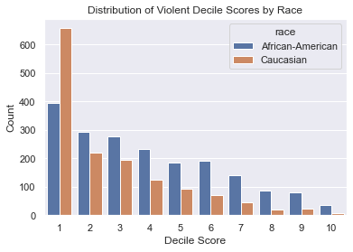
COMPAS violent risk scores also show a disparity in distribution between white and black defendants.
catCols = ['v_score_text','age_cat','sex','race','c_charge_degree']
dfFiltered.loc[:,catCols] = dfFiltered.loc[:,catCols].astype('category')

# dfDummies = pd.get_dummies(data = dfFiltered.loc[dfFiltered['score_text'] != 'Low',:], columns=catCols)
dfDummies = pd.get_dummies(data = dfFiltered, columns=catCols)

# Clean column names
new_column_names = [col.lstrip().rstrip().lower().replace (" ", "_").replace ("-", "_") for col in dfDummies.columns]
dfDummies.columns = new_column_names

# We want another variable that combines Medium and High
dfDummies['v_score_text_medhi'] = dfDummies['v_score_text_medium'] + dfDummies['v_score_text_high']
Regression analysis - logistic regression
formula = 'v_score_text_medhi ~ sex_female + age_cat_greater_than_45 + age_cat_less_than_25 + race_african_american + race_asian + race_hispanic + race_native_american + race_other + priors_count + c_charge_degree_m + two_year_recid'

score_mod = logit(formula, data = dfDummies).fit()
print(score_mod.summary())
Optimization terminated successfully.
         Current function value: 0.372983
         Iterations 7
                           Logit Regression Results
==============================================================================
Dep. Variable:     v_score_text_medhi   No. Observations:                 4020
Model:                          Logit   Df Residuals:                     4008
Method:                           MLE   Df Model:                           11
Date:                Sat, 21 Nov 2020   Pseudo R-squ.:                  0.3662
Time:                        16:26:03   Log-Likelihood:                -1499.4
converged:                       True   LL-Null:                       -2365.9
Covariance Type:            nonrobust   LLR p-value:                     0.000
===========================================================================================
                              coef    std err          z      P>|z|      [0.025      0.975]
-------------------------------------------------------------------------------------------
Intercept                  -2.2427      0.113    -19.802      0.000      -2.465      -2.021
sex_female                 -0.7289      0.127     -5.755      0.000      -0.977      -0.481
age_cat_greater_than_45    -1.7421      0.184     -9.460      0.000      -2.103      -1.381
age_cat_less_than_25        3.1459      0.115     27.259      0.000       2.920       3.372
race_african_american       0.6589      0.108      6.093      0.000       0.447       0.871
race_asian                 -0.9852      0.705     -1.397      0.162      -2.368       0.397
race_hispanic              -0.0642      0.191     -0.335      0.737      -0.439       0.311
race_native_american        0.4479      1.035      0.433      0.665      -1.582       2.477
race_other                 -0.2054      0.225     -0.914      0.360      -0.646       0.235
priors_count                0.1376      0.012     11.854      0.000       0.115       0.160
c_charge_degree_m          -0.1637      0.098     -1.669      0.095      -0.356       0.029
two_year_recid              0.9345      0.115      8.107      0.000       0.709       1.160
===========================================================================================
Black defendants were 77.4 percent more likely than white defendants to receive a higher score, correcting for prior crimes, future criminality.
control = np.exp(-2.2427) / (1 + np.exp(-2.2427))
np.exp(0.6589) / (1 - control + (control * np.exp(0.6589)))
1.7738715321327136